This blog is being built along with a blogging framework for the entire Conundrum ecosystem.
This is taking significantly more time than building a simple blogging website, but when this is complete in a couple months, all users will be able to publish their notes as a blog, independent of any specific service, including Fluster.
On The Gravitational Nature Of Time
Thank you for taking the time to read this. My story is posted elsewhere, so to keep things short, this is the entire reason I built Fluster & Conundrum in the first place. Almost 5 years ago I realized Einstein made an assumption that made far more sense before the observations that give us the Big Bang, and after playing around with the math I realized I can derive an absolutely staggering amount of physics from a single, mathematically equivalent modification to Einstein's model. I quit my job, became homeless, and over the course of this pursuit built the original version of Fluster for my own personal use.
I'll do my best to convince the math types among you (this article does assume some basic understanding of physics and relativity) by the end of this sample note that Einstein made a mistake1, but regardless of your opinions on the model, I hope you enjoy Fluster and find it as useful as I have. Thanks for checking it out!
Included Derivations
Astropy
and
Scipy
. All functions reflect names in the
alpha_omega_gravity
python package, because after 5 years of being homeless I think I earned the right to be grandiose. ( comes from the fine-structure constant).| Derivation | Function | % Error |
|---|---|---|
| cosmological velocity from local gravitational parameters |
vbarCosmological
|
Difficult to assess |
| kinematic velocity from local gravitational parameters |
vbarKinematic
|
|
| Earth's rotational velocity via |
rotationVelocityFromDivergence
|
|
| Solar-Galactic Radius from visible mass |
galacticRadiusPolynomial
|
|
| (solar) |
alphaSolar
|
|
| (Earth) |
omega
,
alphaFactor
|
|
| (orbital velocity) |
solarMetricVelocity
,
vOrbit
|
|
| (from derived velocity) |
vbarAlphaEquivalence
|
|
currentEquivalent
|
||
| from |
omega
,
alpha
|
|
| from |
omega
,
alpha
|
|
| mass density approximation |
massDensityEquivalence
|
|
| as a function of and | -- | |
| Cummulative magnetic diverence at | -- |
.ipynb
notebook and/or install the
alpha_omega_gravity
python package.
Also, keep in mind that if we wanted to be selective we can choose a radius here on Earth's surface that will satisfy many of the above equations perfectly, giving an error of 0. The radii that were used were whichever was most fitting for the job... the mean radius for calculating volume, the polar radius when spin was involved to minimize centripetal influence, and Astropy provided values (equatorial) for everything else.
The Lighthouse & The Clocktower
Consider two observers, and . Let and agree that should travel between two arbitrary points in space2, and at an agreed upon velocity .
At place a time keeping device that remains visible from . Allow that remains at rest relative to , and very near while goes in motion (at an inertial pace) between and .
At what time does observe reach ? If the value is not , but , then , unless . The only possible solution that allows for Einstein's additional factor of while requiring that in the coordinate system of the observer who's kinetic state remains unchanged, and that both and agree upon the time at which reaches is that in the coordinate system of .
To summarize, we have 3 possibilities:
- Every single experimental validation of special and general relativity was flawed. This is statistically almost impossible.
- returns from with a photo of at that disagrees with the photo took of at . There is nothing in physics that prohibits extending the time periods and distances to produce such absurdities as wearing a completely different shirt.
-
elongates by a factor of . We might then presume that this dilation is the source of the equivalence principle, and watch how the physics just lines up.
If you think about it, isn't this inline with what we already believe? Do current models not describe cosmic inflation as a time dependent property? Does more time not pass for the observer in relative motion? Of course and will be further separated, if everything dilates, not just the space in-between galaxies. If we presume that this dilation Einstein applied to time may be applied to space in the coordinate system of the observer in relative motion, then we can describe this spatial dilation as the mechanism to the equivalence principle and combine cosmic inflation, gravitational acceleration and time itself into a single process as observed from different reference frames!
For the physics professionals: Yes, this model violates the Lorentz transformations, but it does so while satisfying every single experimental validation of either SR or GR. Don't stop reading yet, it's just about to get good.
Time Gravity Equivalence
Let's recognize the two primary properties that time occupies:
- A 4th displacement coordinate
-
A driving rate of change
By attributing the 4th displacement coordinate to the density axis that arises from this geometry and the driving rate of change to motion, not time, we can remove our temporal axis entirely! Time becomes nothing more than a mathematical tool... a ratio of other changing properties, all in response to the primary rate of change: motion.
Of course we need to change the dimensionality of much of our physics, but as I will demonstrate here... the math remains remarkably consistent.
Our Cosmological Velocity
Let's consider that this dilation of space might give rise to our gravitational acceleration, where becomes akin to the cosmological rest frame. If we allow that this velocity gives rise to spatial dilation, which then gives rise to the gravitational acceleration that we feel, we should examine the derivative of with respect to .
If we take the average of this integral, we find a scalar product that can be used in the same manner as :
If we solve for , we find:
Substituting the value from equation 2 for we find:
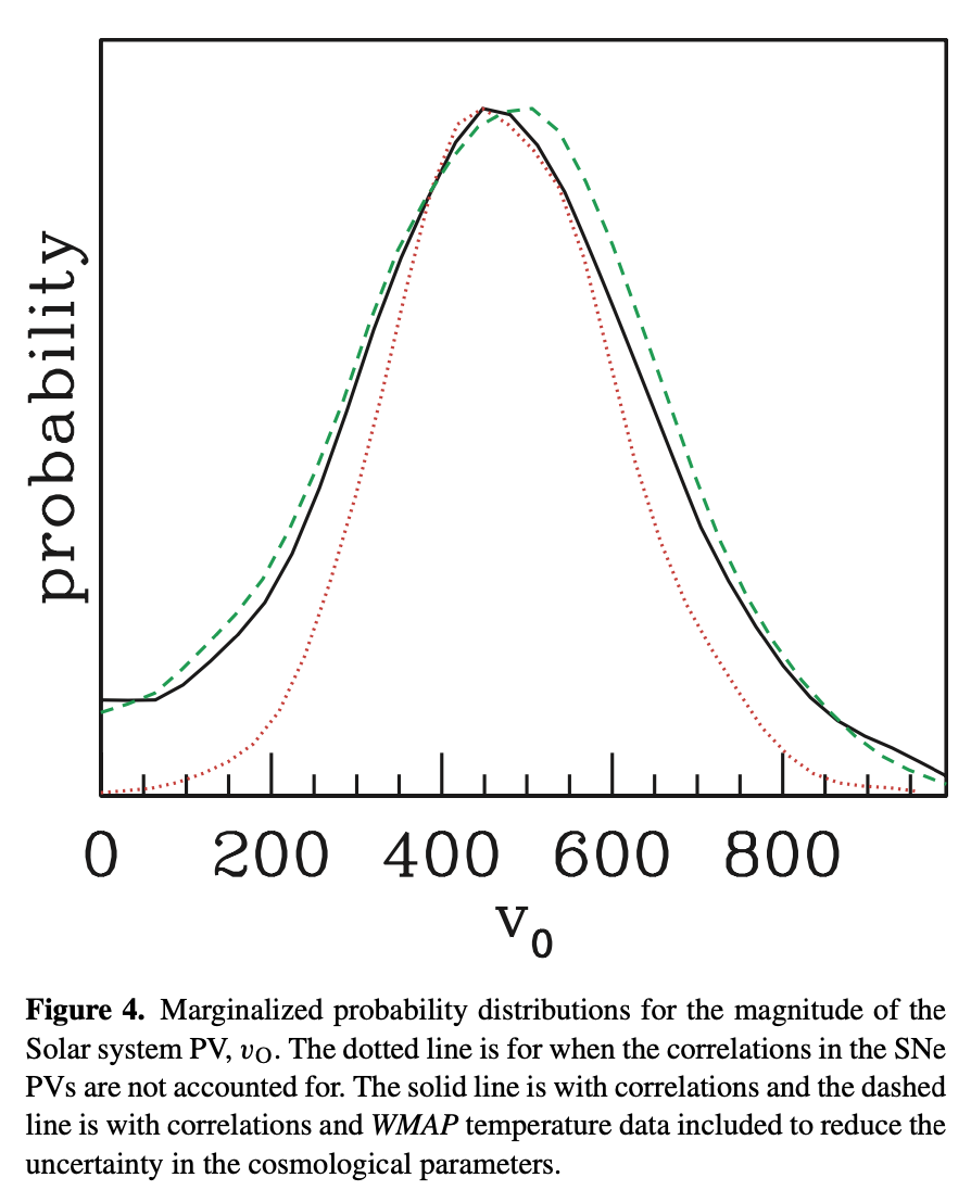
This value coincides closely with direct observation, but due to the wide error margins inherent in these types of observations, we're going to have to do better. Don't worry... we can.
Our Kinematic Velocity
Let's consider the fact that Earth kind of has two velocities, our kinematic velocity (the motion through space), and our cosmological velocity (the motion through space plus the motion of space). Since we just derived our cosmological velocity, we should now remove the temporal axis, giving us a velocity within a contained 3-dimensional 'slice'. This gives a velocity relative to the 'dough' in the common raisin bread analogy of cosmic inflation.
Let's first recognize a time dependent quantity as a dimensionless ratio of distances:
If we consider that time has no driving properties anymore, we should then turn our attention to motion. Since this model proposes that (cosmic inflation and now gravitational acceleration) is time, we can find this time dependent quantity as follows:
Let's then re-examine equation 4 and it's derivation. Since in equation 4 is per unit time, we should then divide by and multiply by our time equivalent quantity from equation 6 .
This gives:
And following the rules of integration defined above, we find:
If we substitute this result back into equation 4 and solve for we find:
Observational ranges for this value that we can observe much more reliably is between , giving us a margin of error of:
Curvature
Note here, that as we integrate , should be elongated by , or . However, this is obviously not what we observe due to our co-motion along our temporal axis. In other words, this integral is applied as a density gradient, inducing a curvature of precisely in the coordinate system of the observer in co-motion.
This means that a linear path in the coordinate system of the 'oven' may be an accelerated trajectory in the coordinate system of the 'dough' due to this intrinsic curvature, should that intrinsic curvature be smooth, continuous, and in our case... radial. This is what allows this steady rate of spatial dilation to produce the appearance of acceleration for a body with no known direct physical interaction; as gravity converts space to time, so too it converts to . This axis acts as a spatial density gradient in the coordinate system of the observer in co-motion who is experiencing these dilatory effects of time, inducing this behavior, but is expressed as Euclidean distance in the coordinate system of the 'oven'.
Where represents this spatial density. at and scales according to where is the radial distance from Earth's surface radius.
This in turn maps , remedying the asymmetry inherent in this model while resolving the issue of terminating geodesics in GR. Blackholes are now nothing more than a mirage in the distance that dissipates as an observer approaches that body's gravitational field.
Interestingly, if we take Earth's radius super-factorial, we find:
Then , approximating Earth's eccentricity.
Let's validate this model by testing this relationship one more time.
Consider the diagram below. If this model is correct, we can improve the derivation of our orbital behavior. Instead of the following:
We can solve this trigonometrically.
Solving this equality for gives only one non-zero solution:
If we substitute in for it's Newtonian value, we find:
As relativity predicts this value does not give 1, but a magnitude slightly higher as .
Plugging this value in to the equation we used to find gives:
This value again coincides closely with our velocity observed relative to the CMB dipole, once again laying credibility to the model we are proposing... gravitational acceleration is a velocity dependent property.
In the relativistic frame
As we used the Newtonian derived orbital parameters in the previous section to derive a relativistic velocity correction in the form of an increase in elapsed 'time', we can now derive a relativistic equation for a body in stable orbit by setting and solving for . This gives a model in the coordinate system of the observer in motion, as he travels at the 'agreed upon velocity' (any velocity multiplied by a scalar of 1).
If we extend our lighthouse & clocktower example to an orbital frame of reference, where orbits at an agreed upon velocity , then this velocity would be decreased by a factor of in the coordinate system of due to the decreased spatial density of , while our relativistically corrected orbital velocity equation becomes as follows:
When we solve for and plugin our galactic parameters here on Earth, we find a radius of , perfectly on top of observational values, without any additional unseen mass!
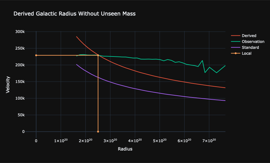
In the plot above, 'standard' is our standard orbital velocity equation , 'derived' is the equation we derived in equation 17 , and 'local' points to our Sun using where is the velocity found by A. Eilers and colleagues, (The Circular Velocity Curve of the Milky Way from 5 to 25 kpc). The actual value we obtain is , without any unseen mass.
Electromagnetism
Consider the determinant of a 3-dimensional, diagonal matrix, representing the change in volume of the coordinate system.
Not only does this accommodate existing experimental validations of SR & GR1, it does so while accommodating the original relativistic experiment: Michelson & Morely23. The only direction they didn't evaluate was along the radial vector, precisely the direction described by this determinant.
If we consider that the magnitude of is this determinant, we should then take it's cube root:
Woah... that number looks familiar that's ! As a matter of fact, when you solve for the
2
, the solution is actually:
Giving a final equation of:
Solving this equation for gives:
That's almost precisely the value we were looking for when we add these values, and almost exactly again when we subtract them, giving very Fibonacci-like vibes.
Using our solar parameters, equivalent to
Let's consider the fact that we have a set of unique properties for two known bodies, us, and the sun. First, we know that all of our observational 'constants' are accurate here. Second, we know that the Sun is the dominant gravitational object in the vicinity. Let's take advantage of this fact by presuming that the lower limit of this 'spinor' approximation is found at the Sun.
Let's consider this function where the , or the same quantity before the torsion applied by and the dilation applied by .
Plugging this back into equation 21 gives:
Where
Demonstrating that this function is more than just a coincidence.
Integrating Magnetic Divergence
Let's now take a second to recognize that to find this quantity
We first took the inverse of divergence. Let's now cube it to bring it back up to scale.
Or expanded, this gives
If we then slide the over to the over side to integrate magnetic divergence according to , we find:
That's
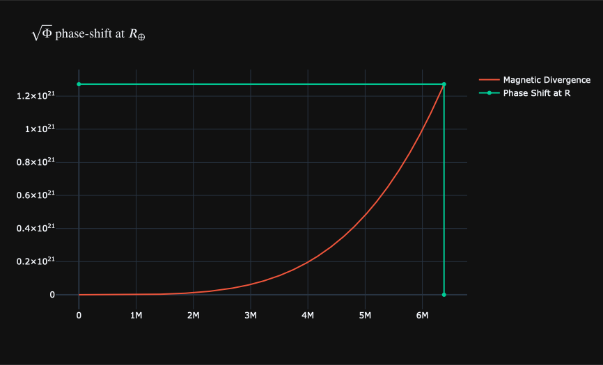
Where the above plot illustrates the intersection of this function with
If you're unfamiliar with physics, let's take a second to break down what we're doing here.
This is what looks like completely written out:
| Component | What it does |
|---|---|
| A consequence of the spherical geometry | |
| The electric constant | |
| The magnetic constant | |
| The fundamental charge | |
| The momentum carrying quantity of a massless photon. | |
| The speed of light, and therefore the speed of causality. |
That's basically the relationship of all of electromagnetism described in one function, now defined in terms of gravitational parameters. Don't worry though, we can keep going! Now that we've derived a relationship to , we can take advantage of the electromagnetic equations. Let's take advantage of the fact that the electromagnetic tensor is undefined at . If electromagnetism can not exist without time, maybe time is masking a subset of electromagnetic properties.
Electric Field Divergence Equivalent
Let's start by assuming the following identity:
Since
then
and
If we then multiply equation 35 by our spinor approximation, converting this linear spatial dilation to rotation, we find:
That's our rotational velocity on Earth's equator ! Off by a total of 0.03 meters (1.18 inches) for a quantity that takes into account a radius the size of Earth's and a period as long as our day!
As in traditional models,
This model uses a velocity that is
When multiplied by our 'time' equivalent , this gives
In the same manner thatVelocity as a function of
Let's consider equation 21 once again. If we re-arrange this equation such that is isolated on one side, we find:
Cubing to bring the units of time back to a power of 1 gives:
If we consider that all velocities are proportional in magnitude to , we should not look for , but for . This then gives:
One can very logically make an argument for the small-angle approximations being a cause for coincidence here, but as a function of ?
Expanding this using our earlier derivation of our cosmological velocity gives
And with some simple algebra, we find:
Displacement Current Equivalent
Let's now consider the electromagnetic displacement current where
Since, in classical electromagnetism:
Then
Or
Note: There is a radius here on Earth's surface where this value is precisely , the Golden Ratio.
Earth's Orbital Velocity From
Consider the radius-independent magnitude of our metric for the dominant body in our system, the Sun:
Considering that nothing in this model is proportional to time, we should consider this model as proportional to , or orbital velocity.
As this relates the dilation of space to the velocity relative to the underlying coordinate system, we should then consider the relationship of static space, and guess what...
Or if approximating as a perfectly circular orbit:
Mass Density Approximation
Finally, let's wrap this all up with one last approximation. Consider the following, that we've derived above:
Then considering that
and the fact that we defined
Then
and
And given the relationship that
and
then finally
This is our observed mass density, ...
That's an error of under 1% for an approximation, that's using approximations and transcendental quantities, demonstrating the wide application of this model.
Results
If we omit this last derivation of , admitting that it is merely an approximation and the derivation of our cosmological velocity, as an accurate estimate is so difficult to obtain, we achieve an average error of , across more than a dozen functions. We've defined as a function of mass density and electromagnetic parameters, we've derived both our kinematic and cosmological velocities, and most importantly... we found as a function of gravitational parameters in multiple, separately defined instances... all using the same principle: elongates by a factor of in the reference frame of , and this is the source of the equivalence principle.
Supportive Arguments
- No terminating geodesics, and no more blackholes. Singularities become nothing but a mirage in the distance that vanishes as you approach that gravitational field.
- The Bullet Cluster observations are heavily indicative of a repulsive gravity model.
- This notion of time paints an entirely different picture of chronology, where there is no limitation on backwards time travel, but a limitation on affecting one's own past. Go back to and try to kill your grandfather. He won't be there anymore as he's now at , if he's still around. Don't get me started on the potentials around massless conciousness in this buoyant, 4-dimensional environment.
- Machian inertia. This model concludes that the Universe is almost precisely as Mach had predicted, with inertia being comprised of the sum of this radiating force for all other bodies in the Universe.
- The entire equivalence principle. We've all become used to it so we overlook just how profound it is, but it's literally assuming what I'm saying is true mathematically and then just pretending it's not in reality.
- The lack of a magnetic monopole, or rather, the existence of an electric monopole. Where do you think that 'sink and faucet' model is funneling charge to? Charge is just space flowing through a hole in an equi-temporal plane, while charged bodies are just bodies with a higher tendency towards one side of this plane due to the buoyant forces along this density axis.
-
Similarly, the induced curvature resolves the paradox produced by the equivalence principle, where a charged particle placed on the surface of a gravitating body does not radiate as if it were in an accelerated frame. This happens because an 'accelerated' frame in the coordinate system of the 'dough' is a linear velocity in the coordinate system of the 'oven'. I intentionally won't use inertial here to describe this path, as the Machian Universe produced by this model does not conserve energy and momentum across this density axis. This apparent violation of the conservation laws follows directly from purely Newtonian mechanics in a dilatory environment.
- This is not a fluke in the math or a mathematical bandaid, this is a core piece of this geometry: This 4th axis is described entirely by spatial density.
- The Fermi paradox. There's an entirely other dimension that life might exist across that we have been so far unable to transcend.
-
Relative motion. Think about it. Do we currently calculate all motion as being truly relative, or do we not already calculate motion as relative to the underlying gravitational acceleration and then lie to undergrads about it? The tensors of GR mask this fact to an extent, but reduce them to their calculus equivalents and we are doing precisely this.